
Understanding kallisto: an interactive guide from reads to abundance
Visits:
RNA sequencing produces millions of short sequences called reads. The challenge is to work backward from those reads and answer two questions: Which RNA transcripts produced them, and how abundant was each transcript? Many transcripts share sequence, so a read often has several possible origins.
kallisto estimates the abundance of each reference transcript from the collective evidence in RNA-seq reads. Using its transcriptome index, it first pseudoaligns each fragment: it determines which transcripts are compatible with the fragment without computing exact alignment coordinates. kallisto then groups fragments with the same compatibility set into equivalence classes and uses the expectation-maximization (EM) algorithm to estimate transcript abundances jointly across the sample.
The examples below let you follow that process. You can change a sequence to see its candidates change, adjust the number of reads to change the evidence, and step through the abundance calculation. After that, we will ask whether a neural network could learn the EM calculation, explore what GPUs can accelerate, and consider why faster hardware may justify revisiting more detailed alignment methods such as Bowtie 2 + RSEM.
- The problem: one fragment, several possible origins
- K-mers: make sequence searchable
- Compatibility classes: group reads with the same candidates
- Why effective length appears
- EM: distribute evidence, then update the estimate
- Could a neural network replace EM?
- What changes on a GPU?
- Research direction: revisit Bowtie 2 + RSEM on GPUs
- Conclusion: two research directions
- References
1. The problem: one fragment, several possible origins
A gene can produce several RNA transcripts through alternative splicing. These versions, called isoforms, share some sequence and differ elsewhere. RNA sequencing, usually shortened to RNA-seq, samples fragments from the RNA population. A read records the sequence at an end of a fragment and may cover only a region shared by several isoforms.
In paired-end sequencing, both ends of a fragment are read. The two reads provide evidence about the same fragment’s origin, so the pair is counted as one observation. The sequence examples below use one read per observation to keep the matching steps easy to follow.
Consider three reference transcripts, labeled T1, T2, and T3. Their sequences are only nine bases long so that every match can be inspected:
T1   ACTGACGTA
T2   ACTGACCTA
T3   GGTGACGTA
The read TGACGTA occurs in both T1 and T3. An alignment describes where a read matches a reference, base by base, including mismatches or gaps. Even a perfect alignment of this read would leave two possible origins. Discarding it would waste evidence; counting it once for T1 and once for T3 would count the same observation twice.
Instead of aligning the read to the reference transcripts directly, kallisto first asks a smaller question: which transcripts are compatible with this read? Finding that candidate set is called pseudoalignment. A statistical model then uses the evidence across all reads to estimate each transcript’s contribution. This separation is central to Bray, Pimentel, Melsted, and Pachter’s original paper.
The reference transcriptome is the collection of transcript sequences supplied to kallisto. Its abundance estimates describe transcripts in that collection; a transcript missing from the reference cannot receive its own estimate.
2. K-mers: make sequence searchable
A k-mer is a stretch of k consecutive bases. Set k to 3, slide a three-base window along TGACGTA, and the read becomes five overlapping windows:
TGA
 GAC
  ACG
   CGT
    GTA
A read of length \(L\) has \(L-k+1\) such windows when \(L\geq k\). An index makes the windows searchable: for each distinct k-mer, it records which reference transcripts contain it. Here, TGA occurs in all three transcripts, while ACG occurs in T1 and T3. A transcript either belongs to that candidate set or does not; repeated occurrences within it do not add extra transcript identities.
Experiment 1 · Sequence → compatibility
Follow a read, one k-mer at a time
Change k or edit the read. Click a k-mer to see its matches and the intersection so far.
Enter 2–60 A/C/G/T bases; spaces are ignored. Sequences are compared in the orientation shown.
Inspect the complete k-mer index
| k-mer | Transcript set C(k-mer) |
|---|
The operation above is a set intersection: retain only the transcripts that appear in every matching k-mer window’s candidate set. Let \(C(\cdot)\) denote a candidate set:
The final answer \(\{T_1,T_3\}\) means either transcript could be the origin. It does not yet assign a probability to either one. Also notice that the five windows still represent one read. They help determine its candidates; they do not become five separate observations in the abundance calculation.
What changing k teaches us
Small k-mers occur more readily by chance. Longer k-mers can distinguish sequences better, but give a short read fewer windows. A single changed base also affects every window that overlaps it.
An absent k-mer is skipped rather than treated as an empty candidate set in this intersection procedure. If none of the windows matches, the read is unassigned. A read is also unassigned when its matching windows point to incompatible sets with no transcript in common. A changed base can sometimes create a match elsewhere in the reference, so surviving matches are evidence rather than a guarantee of the true origin.
For these short examples, k ranges from 2 to 7 and sequences are compared in their written orientation. Real RNA-seq requires attention to read orientation and paired ends. kallisto’s documented index default is k = 31, with an odd-k requirement; those settings are described in the kallisto manual.
Where the graph fits
Notice that several consecutive windows can have identical candidate sets. Once \(\{T_1,T_3\}\) is the running answer, intersecting it with \(\{T_1,T_3\}\) again changes nothing. Avoiding redundant work is one source of kallisto’s speed.
The original index organizes k-mers into a transcriptome de Bruijn graph (T-DBG). K-mers are nodes, neighboring sequence windows connect them, and transcript membership supplies their “colors.” Each transcript follows a path through the graph. Linear stretches with unchanged membership can be compacted into contigs, which may cover only part of a transcript. kallisto uses this structure to skip redundant lookups and checks the end of a skip.
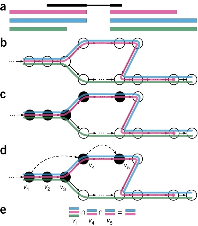
The figure makes the role of contigs concrete. In panel b, each circle is a k-mer and each colored line is a transcript path. Consecutive circles along a nonbranching stretch can be stored as one contig when they carry the same set of transcript colors. In panel d, the dotted arrows show kallisto jumping over k-mers whose candidate set would repeat the same information; the labeled nodes mark lookup points and skip endpoints. Panel e intersects the transcript sets from those informative points to obtain the read’s compatibility set.
The final candidate set has limits: it does not retain the order and positions of every match. With very small k, a string can pass the intersection test even when it does not occur as one continuous sequence in a transcript. This is one reason the choice of k matters.
3. Compatibility classes: group reads with the same candidates
After pseudoalignment, many reads have the same candidate set. Grouping them reduces the data passed to abundance estimation. Three terms describe the successive stages:
- A k-mer compatibility set contains transcripts that contain that k-mer.
- A read or fragment compatibility set contains candidates surviving the combined evidence.
- An equivalence class (EC) groups observations with the same final candidate set. Its count is the number of observations in that group. These are also called transcript compatibility counts (TCCs).
For example, \(\{T_1,T_2\}:90\) means ninety reads could have come from T1 or T2. Their origins are still unresolved. The grouping records one count of ninety, which the abundance model will divide between candidates.
Experiment 2 · Compatibility → counts
Build your own little RNA-seq sample
Each row represents one read sequence observed multiple times. Choose k here and edit the number of copies directly; set the number to 0 to remove that sequence's evidence.
| Read | Copies | T1 | T2 | T3 |
|---|
Only assigned reads enter the likelihood. The button copies your current counts and resets EM with equal effective lengths. Later edits to this sample take effect in EM when you press it again.
What does grouping preserve?
Consider a compatibility matrix as a table with a row for each read and a column for each transcript. 1 means the transcript remains a candidate; 0 means it does not:
The grouped version is \(\{T_1,T_2\}:3\) and \(\{T_1\}:1\). It preserves how often each candidate set occurs, but not the identities or order of the reads that produced those sets. You cannot reconstruct the original labeled table from the counts alone.
For abundance estimation, however, those repeated rows ask the model exactly the same question. A likelihood measures how well a proposed mixture of transcripts explains the observed evidence. Each repeated row contributes the same factor to that likelihood, so multiplying it three times is equivalent to raising it to the third power.
In symbols, let \(\alpha_t\) be the probability that a sampled fragment comes from \(t\), and \(\ell_t\) its effective length, explained next. Let \(e\) denote a candidate set and \(c_e\) its count. Here \(F\) contains the assigned fragments and \(E\) contains their equivalence classes. kallisto’s basic likelihood can be written as:
For the four fragments above, three belong to the compatibility class \(\{T_1,T_2\}\), and one belongs to \(\{T_1\}\). Therefore, their equivalence-class counts are \(c_{\{T_1,T_2\}}=3\) and \(c_{\{T_1\}}=1\). Writing \(g_{12}\) as shorthand for \(g_{\{T_1,T_2\}}\), the fragment-level likelihood \(g_{12}g_{12}g_1g_{12}\) becomes \(g_{12}^{3}g_1\). These equivalence-class counts are sufficient statistics for this likelihood: they retain everything needed to calculate it.
4. Why effective length appears
Imagine two transcripts present in equal numbers of RNA molecules, but one offers twice as many possible fragment starts. It can contribute more fragments simply because it is longer. Fragment share \(\alpha\) therefore differs from the transcript’s share of the RNA molecules.
Effective length accounts for the available fragment starts. For a transcript of length \(L\) and a fixed fragment length \(d\leq L\), a simple effective length is \(\ell=L-d+1\). A 1,000-base transcript with 200-base fragments, for example, has 801 possible starts. Real library models account for a distribution of fragment lengths.
The basic model describes two choices: select transcript \(t\) with probability \(\alpha_t\), then select one of its possible fragment locations. The second choice contributes the inverse-length factor. That is why a compatible transcript contributes \(\alpha/\ell\) to the likelihood term.
With equal fragment shares but effective lengths 100 and 200, a shared observation has relative weights \(\frac{0.5}{100}:\frac{0.5}{200}=2:1\). You can explore this by changing effective lengths in the EM controls experiment.
5. EM: distribute evidence, then update the estimate
Suppose the sample contains many fragments unique to T1 but only a few unique to T2. Dividing every fragment shared by T1 and T2 equally would ignore that imbalance. Evidence from the whole sample should influence the division.
Expectation-maximization (EM) does this in two repeating steps. The E-step uses the current abundance estimate to divide ambiguous evidence. The M-step adds up those assignments and uses the totals as the next abundance estimate. The origin of each ambiguous fragment is the hidden information being estimated.
For a class \(e\), the fraction allocated to a compatible transcript is called its responsibility, written \(w_{e,t}\). It is that transcript’s \(\alpha/\ell\) weight divided by the total weight of the candidates:
Responsibilities within a class sum to one. Multiplying them by the class count divides its evidence without duplicating it. Summing those fractional assignments gives expected transcript counts \(n_t\). The M-step is then:
The M-step simply divides expected counts by \(N\); \(\alpha\) remains a fragment fraction.
A calculation you can reproduce
Take 100 observations unique to T1, 10 unique to T2, and 90 compatible with both. Use equal effective lengths and equal starting weights. T3 has no supporting class here.
The first E-step splits the ninety shared observations 45/45. Expected counts are \((145,55,0)\), so the M-step yields \((0.725,0.275,0)\). The next E-step allocates \(90\times0.725=65.25\) to T1 and 24.75 to T2. Updating gives \((0.82625,0.17375,0)\).
Experiment 3 · Counts → abundance
Be the EM algorithm
Edit class counts, effective lengths, and initialization
Change the evidence or the starting estimate to see how EM responds. Effective lengths are independent of the short sequences in experiment 1. Any edit restarts EM.
| Transcript | Effective length ℓ | Starting weight |
|---|
Starting weights are normalized to sum to 1. Keep them positive so a possible transcript is not permanently excluded.
The animation restarts from the selected initial weights. It shows the early cycles, then uses representative checkpoints when convergence takes many iterations.
| Transcript | α | N × α | TPM |
|---|
| Class (count) | To T1 | To T2 | To T3 |
|---|
Each row sums to its class count. The M-step divides each column total by N to get the next α.
This experiment stops when the largest change in a transcript's fragment share is below \(10^{-8}\), with a limit of 2,000 updates per run. kallisto uses its own convergence criteria.
In this example, the final T1:T2 ratio is set by the unique evidence: \(100:10\). Running EM to convergence gives approximately \((0.90909,0.09091,0)\). The ninety shared fragments add to the estimated counts but cannot distinguish those two transcripts by themselves.
Why estimated counts and TPM differ
Fractional assignments naturally give noninteger estimated counts. Once EM has fit the fragment shares, the estimated count for a transcript is \(N\alpha\). To account for transcript length, divide these counts by effective length and scale the resulting shares to a total of one million. The result is TPM, or transcripts per million:
TPM sums to one million when the total is positive. It equals \(\alpha\) multiplied by a million only when the effective lengths are equal. Compare the \(\alpha\) and TPM columns after changing the lengths: they answer different questions about the same sample. At iteration zero, \(N\alpha\) is only an initial guess; after fitting, it is an estimated fragment count rather than a direct count of original RNA molecules.
Can a stable answer still be ambiguous?
Select Unidentifiable. Only \(\{T_1,T_2\}\) appears, and the effective lengths are equal. No observation distinguishes the two transcripts. Once \(\alpha_3=0\), the likelihood depends on \(\alpha_1+\alpha_2\), so every split with that sum equal to one fits equally well.
This is a lack of identifiability: the evidence does not determine a unique answer. More reads from exactly the same shared class cannot resolve it; distinguishing reads or additional assumptions are needed. A stable optimizer is therefore only one part of interpreting an abundance estimate.
The sections so far cover kallisto’s core path from reads to abundance. The remaining sections use that foundation to ask how learned surrogates and modern GPUs might change the algorithm.
6. Could a neural network replace EM?
Neural networks are increasingly used in scientific computing to approximate calculations that would otherwise require an expensive numerical solver. Such a network is often called a surrogate model: it is trained on input–output examples from the original calculation and then learns a faster approximation to that mapping. A prominent example is the Fourier Neural Operator, which learns mappings from the inputs of partial differential equations to their solutions across a family of problems, rather than solving each instance independently from the beginning.
Transcript quantification suggests a related opportunity. After pseudoalignment has reduced the reads to equivalence-class counts, EM repeatedly redistributes those counts and updates transcript abundances until convergence. The 2026 GPU kallisto study makes the remaining cost visible: in its average timing breakdown, GPU mapping takes 722 ms while EM takes 3,148 ms. Accelerating k-mer lookup therefore exposes abundance estimation as a major part of the computation.
There is already research connecting neural networks and EM. Neural Expectation Maximization constructs a differentiable EM-like procedure in which a neural network learns the statistical model used for perceptual grouping. UNEM takes another route: it unfolds the iterations of a generalized EM algorithm into network layers and learns iteration-specific parameters for few-shot classification. Neither paper studies RNA-seq, but both show that the repeated structure of EM can be exposed to learning.
This raises a research question for transcript quantification: can a neural network learn the EM computation that maps equivalence-class evidence to transcript abundances?
7. What changes on a GPU?
Modern GPUs can run thousands of small operations at the same time, and their memory bandwidth has increased along with their computing power. kallisto contains work that can be separated naturally: different fragments can look up k-mers independently, different candidate sets can be intersected independently, and different equivalence classes can contribute to an EM update in parallel.
A coauthor revisits kallisto on a GPU
In the March 2026 preprint RNA-seq analysis in seconds using GPUs, Páll Melsted, a coauthor of the original kallisto paper, joins Elís Mar Guðnýjarson and Jóhannes Nordal in redesigning pseudoalignment, equivalence-class intersection, and EM for NVIDIA GPUs. Across 100 Geuvadis RNA-seq samples, they report about a 30× speedup when setup is excluded. For a dataset containing 295 million paired-end reads, runtime falls from about 40 minutes with 16 CPU threads to 50 seconds on the GPU.
Their benchmark results are reproduced below:
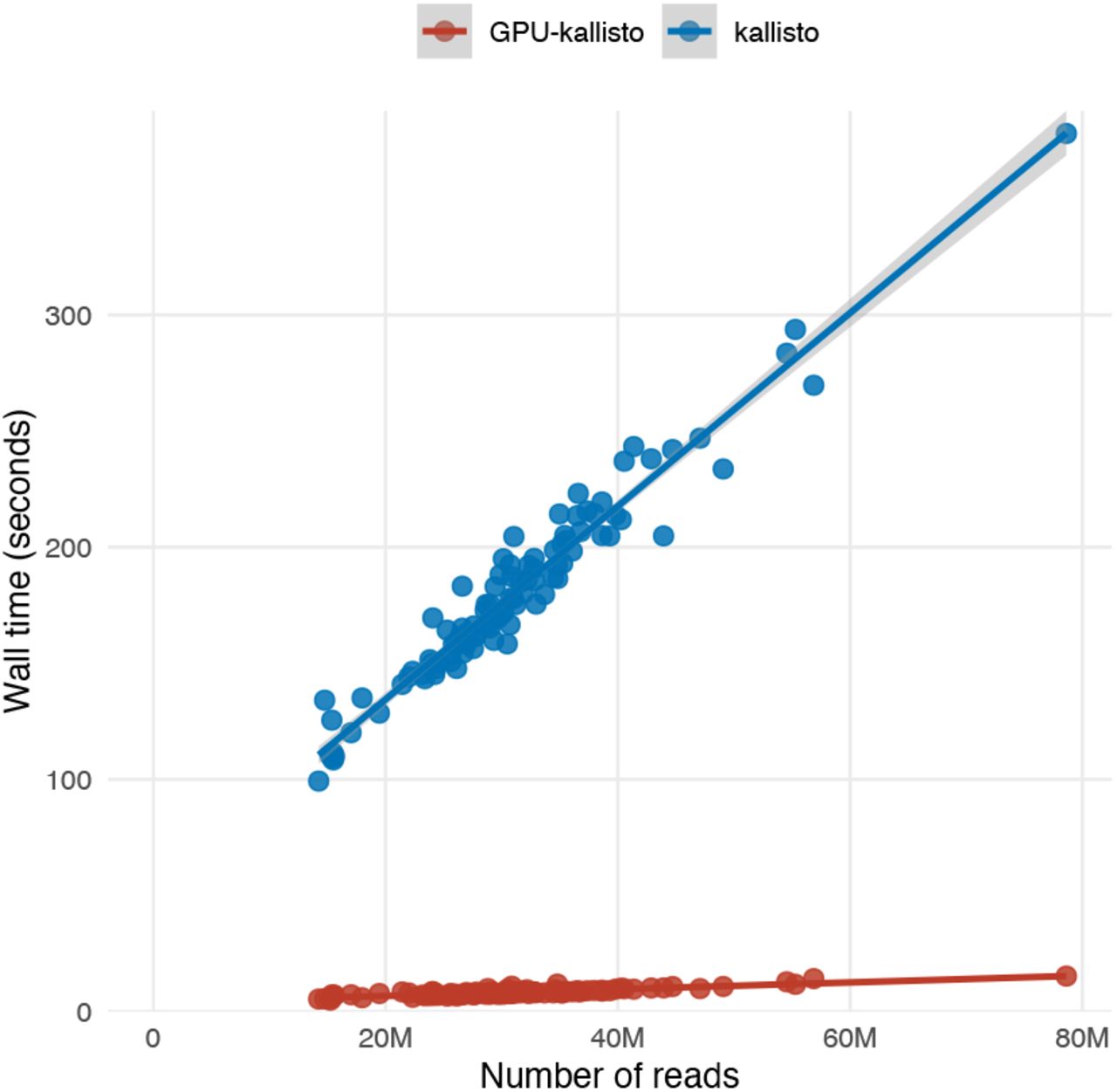
The benchmark used an RTX 5090 with 32 GB of GPU memory, a Ryzen 9 9900X, NVMe storage, and BGZF-compressed input. BGZF divides compressed data into independent blocks, allowing several blocks to be decompressed on the GPU at once; ordinary gzip remains serial and is decompressed on the CPU.
How they implement it: k-mers and EM in parallel
The transcript index is moved into GPU memory. Each k-mer is encoded as a 64-bit integer and looked up in a GPU hash table to obtain an equivalence-class ID. Transcript sets are stored in one flattened array with offsets marking where each set begins. Threads generate and look up k-mers from many reads concurrently, remove repeated and empty candidate sets, intersect the remaining transcript lists, and look up the resulting equivalence class.
The intersections have different sizes, so their memory requirements are not known in advance. The implementation first estimates how much temporary space each read needs, uses a parallel prefix scan to assign each thread a nonoverlapping slice of memory, and then performs the intersections in a second pass. This two-pass design replaces the convenient per-read dynamic allocation that a CPU implementation might use.
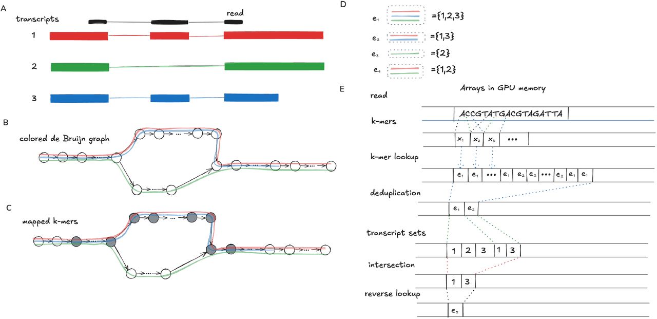
EM uses a second layout: a transposed index records, for each transcript, every equivalence class containing it. During the E-step, the GPU first calculates the denominator for every class in parallel. It then uses the transposed index to sum class contributions for every transcript in parallel. The M-step normalizes those transcript totals, and the implementation checks convergence every ten iterations. This is the same E-step and M-step from Experiment 3, reorganized so that a single iteration can occupy the GPU.
Implementation details are available in the kallisto GPU branch.
What is the bottleneck now?
The paper reports a mapping rate of 24.1 million read pairs per second, but an end-to-end rate of about 3.6 million pairs per second. In its average timing breakdown, GPU mapping takes 722 ms while EM takes 3,148 ms. I/O and decompression use another 841 ms of GPU time plus 2,370 ms of CPU time. Once k-mer lookup becomes this fast, it is no longer the main constraint.
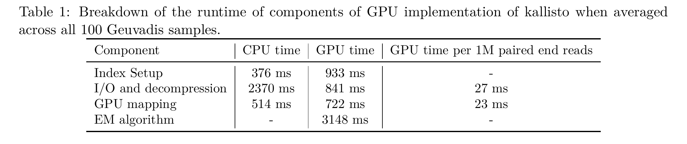
This result shifts the research question from “Can kallisto run on a GPU?” to Should the saved computation be used to obtain richer evidence, rather than only to reduce runtime? If pseudoalignment is no longer expensive, selected ambiguous fragments could receive additional alignment or sequence-error scoring before abundance estimation. This possibility leads directly to reconsidering Bowtie 2 and RSEM below.
8. Research direction: revisit Bowtie 2 + RSEM on GPUs
The GPU result suggests a broader question: if pseudoalignment is now extremely fast, is discarding alignment detail still the best accuracy–runtime tradeoff? kallisto keeps candidate-transcript sets, whereas Bowtie 2 preserves base-level alignment evidence and RSEM uses that evidence to estimate expression. Modern GPUs may make it practical to retain more information without returning to the runtimes that originally motivated pseudoalignment.
Bowtie 2 + RSEM was a strong accuracy baseline in the original kallisto comparison, but that does not establish it as universally more accurate. Later work also shows that mapping methodology affects abundance accuracy on real data. The research question is therefore whether richer alignment evidence improves transcript estimates enough to justify its remaining computational cost, particularly for rare and highly ambiguous isoforms.
A rough study would have three stages. First, accelerate Bowtie 2–compatible alignment while preserving the paired-end relationships, alignment scores, and record formats that RSEM requires. Second, parallelize RSEM’s abundance estimation without changing its statistical model. Third, compare this pipeline with GPU kallisto on the same references and RNA-seq libraries, measuring end-to-end runtime, memory use, and gene- and transcript-level accuracy using both simulated truth and independent experimental evidence. The result would test whether modern hardware changes which information should be retained for transcript quantification.
9. Conclusion: two research directions
kallisto became fast by asking only which transcripts are compatible with each fragment, compressing repeated candidate sets into equivalence-class counts, and applying EM to estimate abundance. The experiments in this article expose both sides of that design: compression makes computation efficient, but shared fragments can remain unresolved, and EM still requires repeated updates.
Two research directions follow from this tension:
- Learn the abundance calculation. A neural surrogate could operate on the graph connecting equivalence classes and transcripts, learning several EM-like updates or directly approximating the converged abundance estimate. This direction asks whether the repeated computation can be learned while preserving the likelihood objective and correct behavior when the evidence is ambiguous.
- Retain richer evidence with GPU computing. A GPU implementation of Bowtie 2 + RSEM could preserve alignment locations, scores, mismatches, and paired-end constraints that pseudoalignment omits. This direction asks whether modern hardware can make a more detailed statistical model competitive in runtime and more informative for rare or ambiguous isoforms.
These directions spend computation differently. One learns a faster solver after the evidence has been compressed; the other keeps richer evidence and accelerates the full pipeline. Testing both on the same data would show whether the next improvement comes from faster inference, better evidence, or both.
10. References
- Bray, N. L., Pimentel, H., Melsted, P., and Pachter, L. (2016). Near-optimal probabilistic RNA-seq quantification. Nature Biotechnology, 34, 525–527.
- Pachter Lab. kallisto manual.
- Li, Z., Kovachki, N., Azizzadenesheli, K., Liu, B., Bhattacharya, K., Stuart, A., and Anandkumar, A. (2021). Fourier Neural Operator for Parametric Partial Differential Equations. International Conference on Learning Representations.
- Greff, K., van Steenkiste, S., and Schmidhuber, J. (2017). Neural Expectation Maximization. Advances in Neural Information Processing Systems, 30.
- Zhou, L., Shakeri, F., Sadraoui, A., Kaaniche, M., Pesquet, J.-C., and Ben Ayed, I. (2025). UNEM: UNrolled Generalized EM for Transductive Few-Shot Learning. Proceedings of CVPR, 9665–9675.
- Melsted, P., Guðnýjarson, E. M., and Nordal, J. (2026). RNA-seq analysis in seconds using GPUs. bioRxiv, version 1.
- Pachter Lab. GPU branch of kallisto. Source code accompanying Melsted et al. (2026).
- Langmead, B., and Salzberg, S. L. (2012). Fast gapped-read alignment with Bowtie 2. Nature Methods, 9, 357–359.
- Li, B., and Dewey, C. N. (2011). RSEM: accurate transcript quantification from RNA-Seq data with or without a reference genome. BMC Bioinformatics, 12, 323. See also the RSEM alignment requirements.
- Srivastava, A., Malik, L., Sarkar, H., Zakeri, M., Almodaresi, F., Soneson, C., Love, M. I., Kingsford, C., and Patro, R. (2020). Alignment and mapping methodology influence transcript abundance estimation. Genome Biology, 21, 239.